Artificial Neural Networks
Predictive methods can be divided fundamentally in Numerical Weather Prediction (NWP) models and statistical techniques. Time series prediction belongs to statistical techniques group, which is based on obtaining future values of the variable to predict in function of past observations.
Artificial Neural Networks (ANNs) paradigm was originally an abstract simulation of neural biological systems which tried to synthetic its abilities [3].
Supervised training networks have been the neural network models more developed from the beginning of its design. Training data is constructed by various input and output patterns. Knowing the output is a fact from which the training benefits as a master which supervises and modify its parameters.
Neural network used is backpropagation type; this class of supervised network has a learning algorithm based on error correction method. Learning in backpropagation networks is done in the following way: an input pattern is selected from the set of input patterns, it determines the activations of input nodes, latter, neurons are activated from hidden layers and finally output units are computed. The activation pattern which links the output layer is then compared with output pattern associated to the input pattern to calculate the error [4].
The methods described in the previous section are trained with 75% of the data set. Assessment of the models proposed is performed over the 25% of the clearness sky separated sequentially for this purpose.
Neural Network (NN) is essayed with different layer sizes and neurons in each layer with the following architecture:
• One layer and one neuron.
• Two layers with three neurons in input layer and one neuron in output neuron.
• Three layers with five neurons in input layer, three neurons in hidden layer and one neuron in output neuron.
• Four layers with eight neurons in input layer, five and three neurons in hidden layers and one neuron in output neuron.
• Five layers with fifteen neurons in input layer, eight, five and three neurons in hidden layers and one neuron in output neuron.
Training algorithm is Leverage-Marquardt algorithm [3].
 |
||
Accuracy of each one of the models presented is studied in terms of relative Mean Bias Deviation (MBD) and Root Mean Squared Deviation (RMSD):
being N the population size, Kt clearness sky index observed and Kt half daily clearness index predicted.
Each one of the models essayed is compared with a basic model, persistence model (PER), which is based on assumption that clearness index for next temporal step is the same as last temporal observation. Comparisons are done in terms of relative RMSD. Improvements over persistence for deviation index (i-error) (in terms of RMSD) defined previously, is obtained from the following expression:
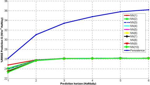
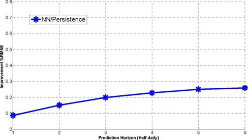
The neural network model, NN(z), has been tested with different input vector size which represents the temporal value of the difference of lost components for half daily lags z=1..10. Fig 4. shows results for percentage of error in term of RMSD for NN model with just one neuron and one layer and with different input vector size. Improvement of the model with lower RMSD (NN(10)) against persistence is shown in Fig. 5. Difference of lost component time series is a signal with high variability which can be seen in the results in the fact that from second time step of prediction the error gets an upper limit of approximately 26% of RMSD.
|
Fig. 4. RMSE Error: model NN with [1] layer and only lost component as input. |
|
Fig. 5. Improvement NN(10) over Persistence: NN with [1] layer and only lost component as input. |
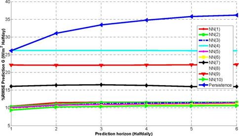
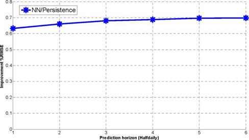
The second model essayed is based on using as input vector the synoptic situation difference for the time step which is being predicted and the difference of lost component for half daily lags z=1..10. Fig 6. shows results for percentage of error in term of RMSD for NN model with four layers and eight,
|
|
|
|
|
Properties of ground global solar radiation has been presented based on requirements of statistical prediction techniques. The solar radiation time series has been transformed taking into account gaussian and stationary properties needed by neural network model used to predict future values.
A new model to predict time series of ground global solar radiation based on previous transformation of solar radiation time series has been presented. The error of the model is limited by an upper level which is due to deterministic nonlinear behaviour of the signal that can’t be followed correctly by neural network model. The second model presented is based on using the difference of lost component and the difference of the synoptic situation for the time step of prediction. The error has a lower level of nine percent. The neural network used has a structure more complex than the network used in previous works.
[1] Veziroglu TN and dot a. 21st Century's energy: Hydrogen energy system. Energy Conversion and Management 2008; 49:1820-1831.
[2] Patlitzianas KD, Ntotas K, Doukas H, and Psarras J. Assessing the renewable energy producers' environment in EU accession member states. Energy Conversion and Management 2007; 48:890-897.
[3] Haykin S. Neural networks. A comprhensive foundation. New York (USA): 1994.
[4] Palit AK and Popovic D. Computational Intelligence in Time Series Forecasting: Theory and Engineering Applications. 2005.


